1. Introduction
Taxes are not always beared by the agent designed to do so by scal authorities. Economic analyses consider this at least since Quesnay (1759) explained that each and every tax of the French ancien rйgimе is eventually beared by landlords. Afterwards, dierent bearers for dierent taxes has been considered by Smith (1776) then Ricardo (1821) (e.g.: luxury good consumers, landlords, capitalists at least for the share of prot which is not constituted by risk premium) then the question of tax incidence has become a major issue of economic analysis. The present article generalyses existing economic litterature on consumption tax incidence to general forms of consumption taxes. Previous studies were limited to the cases of per unit and ad valorem taxes.

Three main contributions are provided. From a methodological point of view, the elasticity of the tax function is introduced as a new parameter to take the shape of general consumption tax schedules into account in dierent models of imperfect competition in a tractable manner. From a theoretical point of view, existing results on the dierence of incidence of ad valorem and per unit consumption taxes are generalized to non-linear consumption taxes: the larger the elasticity of the tax function the weaker the share of the consumption tax beared by consumers.

From an applied public economic point of view, it is shown how the regulator may put downwards prices on very uncompetitive markets by increasing the elasticity of the consumption tax on a targeted window of producer prices.
The incidence of consumption taxes is of main importance as much for equity reasons as for eciency ones. It measures the way a tax burden is shared between dierent economic agents (producers and consumers in the case of consumption taxes), which determines the distributive impact of scality. It also measures the way consumptions taxes impacts the total output, and therefore the deadweight loss of indirect taxation. Standart results are that consumers bear the whole tax burden in perfect competiton in the long run, but that it may be shared with producers in the short run or when competition is imperfect (e.g.: Fullerton and Metcalf (2002)). In that case, the consumer share of the tax burden decreases with respect to the demand elasticity and increases with recpect to the elasticity of the marginal cost of production (e.g.: Carbonnier (2009)). Furthermore, tax incidence depend on the structure of competition, and the consumer share may even be greater than 100%. This has been conrmed theoretically by Stern (1987); Besley (1989) for homogenous products and Anderson et al. (2001a,b) for heteregenous products; it has been also empirically conrmed by Besley and Rosen (1999) and Carbonnier (2007, 2009, 2011).

Furthermore, the form of the tax itself in uence its incidence. This has been noticed early in the economic literature. At the begining of the XIXth century, Cournot (1838) allready found a dierence between incidencesof unit and ad valorem consumption taxes under monopoly. Since, only these two kind of consumption taxes has been studied. If these two taxes are equivalent under perfect competition, the literature has shown that consumers bear a large share of unit taxes than ad  valorem  taxes.  Wicksell  (1896)  demonstrated this result in the case of a monopoly with constant marginal costs, Suits and Musgrave (1953) for all monopolies, Delipalla and Keen (1992) under Cournot oligopoly with conjectural variations and Anderson et al.  (2001b)  under  Bertrand  oligopoly.  This result has been empirically conrmed by Delipalla and O'Donnell (2001) and Carbonnier (2011) using respectively the european tabacco market and the French alcohol market.

The intuition behind this very general result is quite simple. Whatever the producer price, the amount of the tax per unit of output is the same. However, the tax itself decreases if the producer decreases its own price in the case of ad valorem consumption taxes. Threfore, ad valorem consumption taxes subsidies the producer price decreases, adding a tax decrease to the producer price decrease. This incentive make price decreases more protable for producer in the case of ad valorem consumption taxes, and leads to lower consumption prices for the same level of tax revenue.

However, these two kind of taxes are not the only possible ways for taxing consumption, and more complex schedules might be setted. For existing exemple, the French tax on oil (TIPP for Taxe  a l'Importation sur les Produits P  etroliers) was settle with a special schedule between October 1st 2001 and July 21 2002. It was a per unit tax whose value decreases with respect to the values of the Brent baril (oating TIPP). For potential exemple, European tax systems uses different VAT rates for different goods. Mainly, all countries have at least a full rateand a reduced rate, this last for different goods and services among whom ఇrst necessisty consumption. However, if ordinary meat is considered as ఇrst necessity consumption, it should not be the case of luxury meat, and the government may want to tax meat at different rate (full or reduced) depending on its price.

The intuition about the per unit/ad valorem result puts forward the importance of the variation of the tax with respect to the producer price. The present article propose a usefull parameter to measure it: the elasticity of the tax function. Different model of imperfect competition are derived according to understand the impact of this parameter on the incidence of consumption taxes.

The remainder of the article is compose as follow. Section 2 introduces the elasticity of the tax function, and gives some exemples of its value for different existing or potential consumption taxes (2.1). Then, the theoretical methodology is presented (2.2), with exemples concerning perfect competition and monopoly: the elasticity of the tax function has no impact on tax incidence under perfect competition, but the consumer share of the tax burden decreases with respect to it. Section 3 shows the same result in the case of markets for homogenous goods, both in the short run (3.1) and in the long run (3.2). Section section 4 analyses the case of markets for heterogenous goods. The result stands in the short run (4.1) but not always in the long run (4.2). Section 5 concludes, discuss the consequences in matter of welfare and optimal taxation and draws the perspective for further studies.

2. Theoretical framework

The introduction presented the intuition behind the incidence difference between per unit and valorem consumption taxes. The key property is the way the tax itself varies when the producer price varies. Indeed, ad valorem consumption taxes induces lower consumer price than unit taxes because the unit tax is independant from the producer price when the ad valorem tax increases with respect to the producer price. Therefore, ad valorem taxes generate a larger incentive for producers to decrease their price, because it decreases also the amount of tax due.

This property of the consumption tax should be synthetized in a parameter which could be introduced in models of market equilibrium. In that purppose, the present section introduces such a parameter: the elasticity  of  the  tax  function.  The  first  subsection presents this elasticity asa well as exemples of non-linear consumption taxes.

The following subsection presents the theoretical strategy as well as exemples concerning perfect competition and monopoly.

2.1. The elasticity of the tax function

First of all, the consumption tax function T is defined as the function giving the consumer price q from the producer price p (the 
actual tax being the difference between the two). It allows to consider every kind of consumption tax.

For exemple, the per unit tax function is T(x) = x + t where t is the actual tax per unit and the ad valorem tax function is T(x) = (1 +τ)τx where τ is the actual rate of ad valorem consumption tax. Given this tax function, the key parameter about the form of the consumption tax is the elasticity of consumer price to producer price.

This elasticity gives the curvature of the tax function. For ad valorem consumption taxes, this elasticity is equal to one:

For per unit consumption taxes, this elasticity is lower than one:

In addition, other kind of consumption taxes are possible, even if no scal system has adopted them yet. A piecewise proportionnal consumption tax would have an elasticity equal to one except at the price threshold for the coecient change where it is equal to infinity. Consumption taxes with a polynomial shape T(p) = Ap^β  have elasticity equals to β:

Therefore, the consumption tax may increase strongly with respect to the producer price if β > 1. The extreme case is the exponential consumption tax q = Ae^p whose elasticity is equal to p:

At the opposite, it may be chosen that the consumption tax is used to minimize the producer price volatility with an elasticity inferior to 1, it is the cas of polynomial consumption taxes with β lower than one.

Furthermore, the exemple of non-linear presented in the introduction may be explorated in this context. Let say for exemple that government want to tax at reduced rate meat under ten euros per kilogram and at the full rate above forty. Between, the tax rate may be linear increasing or smoothly increasing (the actual exemple consider a cubic function of the producer price). Figure 1 shows these two consumption taxes and their elasticity.

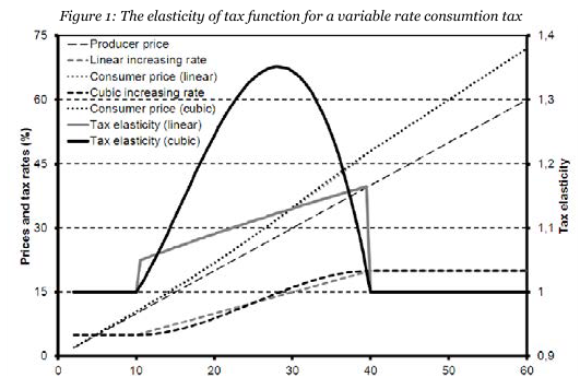
It appears that these taxes – reduced rate for low prices and full rate for high prices - presents elasticity of the tax function signicantly above one between the threshold of end of reduced rate and those of begining of full rate.

This eslasticity of the tax function matters between it gives the link between consumer preference and variations of the producer price. Indeed, consumers behavior depend on their consumption and their budget constraint.

Therefore, from their preferences derives the elasticity of demand with respect to the consumer price ∈_q. However, the behavior of the producers depend on the reaction of the demand to changes in the producer price ∈_p. The relation between the two elasticities of the demand is given by equation 1.

Indeed, .

It is how the elasticity of the tax function is inserted into the different models.

2.2. Theoreticall methodology

In the following of the paper, a strategy is adopted to understand the inuence of the shape of the tax function – the elasticity of the consumer price to the producer price. First of all, a given equilibrium E₀ is considered with a producer price p₀, a consumer price q₀ = T₀(p₀) and a quantity produced Y₀. Then, the shape of the tax function is changed as T₁ in a such way that the new equilibrium E₁ has the same consumer price q₁ = q₀ = q than E₀. It should be notice that at this new equilibrium, the quantity produced on the market is  Y₁  =  D(q₁)  =  D(q₀) = Y₀  = Y; hence, the marginal cost of producers and the demand elasticity are the same at the two equilibria.

The only variables that may change because of the change in the shape of the tax are the producer price p₁ and consequantly the tax revenue F₁ = Y (q – p₁) ≠ Y (q  – p₀) = F₂. If p₁ > p₀, then F₁ < F₀ and the change in the form of the tax decreases the eciency of the consumption tax: for the same quantity produced and the same consumer price, the tax revenue is lower, or reciproquely, for the same tax revenue, the consumer price is larger and the quantity produced lower. For reciproqual reasons, if p₁  <  p₀, then  F₁ > F₀ and the change in the shape of the tax increases the eciency of the consumption tax. Some results may be derived immediatly.

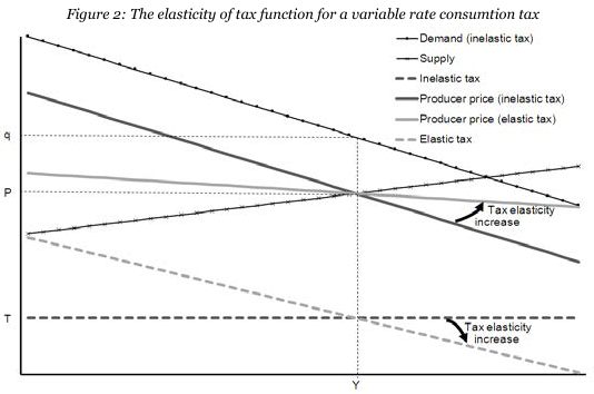
Very simple exemples of this methodology are given by the study of the two polar cases of perfect competition and monopoly. Figure 2 shows the case of perfect competition.

Under perfect competition, the output Y is given by the intersection of the producer price (solid dark grey) and the marginal cost (thin crossed black line), the consumer price (thin dotted black line) being the inverse demand for this output. Changing the tax function  T₀ for another T₁ more elastic but with the same output at equilibrium consists in drawing a new producer price curve (solid light grey) with a lower shape but cutting the marginal cost curve for the same value of output Y. Consequently, the producer price does not change: p₁ = C_m(Y ) = C_m(Y₀) = p₀ and neither does the tax revenue.

Proposition 1. Under perfect competition, a change in the consumption tax such that the elasticity ∈_T increases but the consumer price stay unchanged leads to:

(a) no change of the producer price

(b) no change in the fiscal revenue

However, the shape of the tax actually matter regarding the incidence of consumption taxes under imperfect competition. The polar case of monopoly is presented by figure 3.

The monopoly output Y is given by the intersection of the marginal cost (crossed line) and the marginal revenue (solid dark grey), itself derived from the producer price curve (dashed dark grey); the consumer price (thin dotted black line) being the inverse demand for this output. Changing the tax function T₀ for another T₁ more elastic but with the same output at equilibrium consists in drawing a new marginal revenue curve (solid light grey) with a lower shape but cutting the marginal cost curve for the same value of output Y. Consequently, the consumer price does not change:  q₁ = D^–1(Y ) = D^–1(Y₀) = q₀ and neither does the marginal cost of production. However, the producer price curve changes (dashed light grey) and so does the actual producer price and therefore the tax revenue.  Figure 3 shows that an increase of the elasticity of the tax function leads to a decrease of the producer price and an increase of the tax revenue.

Proposition 2. On a monopoly market, a change in the consumption tax such that the elasticity ∈_T  increases but the consumer price stay unchanged leads to:

(a) a decrease of the producer price

(b) an increase of the tax revenue

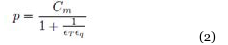
Proof.  The  producer  price  verifies the Lerner condition:  where ∈_T is the elasticity of the demand with respect to the producer price p. However, the demand function depends on the consumer price q and the demand reaction parameter should be the elasticity of the demand with respect to the consumer price ∈_q. Given the relation between shown by equation 1, the producer price of a monopoly is given by equation 2.

 As the quantity Y and the consumer price q are the same in E₀ and E₁, the values of the marginal cost of production and the 
elasticity of demand with respect to the consumer price are also the same. Therefore, the difference between p₀ and p₁ comes only from the difference between ∈T₀ and ∈T₁. The quantity produced and the consumer price being equal, the producer price decreases with respect to the elasticity of the consumption tax ∈_T . Q.E.D.

The consumer share in the tax burden decreases with the elasticity of the tax; the producer share increases.

This result generalizes Suits and Musgrave  (1953)  for  a  general  form  of consumption taxes as the elasticity of per unit consumption taxes is lower than the elasticity of ad valorem consumption taxes.

3. Homogenous goods

This section aims at understanding the in؍uence of elasticity of the tax function on the incidence of consumption taxes in the case of imperfect competition. It focuses on the matter of quantity and price, the following section studies the question of quality. But before considering the diversity of consumption, this section analyses production of homogenous goods. In that case, Bertrand competition leads to equilibria where the producer price is equal to marginal cost of production. The consequence regarding the purpose of the present paper is that elasticity of the tax function has no impact on consumption tax incidence, as it is the case under perfect competition.

Therefore, imperfect competition in market for homogenous goods is analysed in a Cournot oligopoly model.

Such models have been criticed under argument that quantity competition is less credible than price competition.

However,  pure  Bertrand  competition assumes production follows directly demand without capacity constraints.

Furthermore Kreps and Scheinkman (1983) shows that a game where ֝rms invest in stage one (implying capacity constraints 
for the second stage) then price competition occurs in the second stage gives the same output and prices as Cournot competition. See Tirole (1988) for discution of the KrepsScheinkman game and Wu et al. (2012) for its extension to the case of non concave demand.

The present section is based on the Cournot oligopoly model with conjectural variations developped to take into account the possibility of collusion and free entrance on market. It is the Cournot oligopoly model used by Katz and Rosen (1985); Stern (1987); Besley (1989) to evualuate consumption tax tax  incidence,  then  by  Delipalla  and  Keen (1992) to shows the difference of incidence of unit and ad valorem consumption taxes and Carbonnier  (2009)  to  show  the  df֝erence of consumption tax shifting upwards and downwerds in the short run. To understand speci֝cally the effect of entry in the market, the  ֝rst  subsection  considers  a  closed oligopoly then the second one allows for free entry.

3.1. Closed oligopoly

Let us consider n  ֝rms  with  the  cost function  C(y_i) where C(0)  =  K  is  the  ֝xed cost.  Each  firm  anticipate  the  reaction  of its competitiors such as . Therefore, Cournot-Nash oligopoly corresponds α  = 0.

Parameter  α measures the collusion on the market: with the model is equivalent to perfect competition and with  α = 1 it is equivalent to monopoly. The model is solved at the symmetric equilibrium. Hence, the overall change in production anticpated by each ֝rm is then given by equation 3.

Parameter  γ  =  α  +  (1  –  α)  /  n  measure the degree of competition in the market, the model is equivalent to perfect competition if γ = 0, to Cournot-Nash oligopoly if and to monopoly if γ = 1. It means that firm i anticipate a production Y₀ if it exists the market, and that the total output is  Y = Y₀ + γny_i if it produces y_i. The profit of a firm is given by equation 4.

For choosing the level of production that maximizes its profits, the firms anticipates a price variation due to their output variation such as in equation 5.

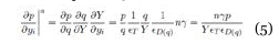
Therefore the first order condition of the profit  maximization  is  given  by  equation  6 and the second order condition is given by 7.

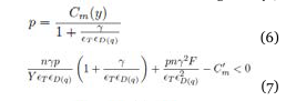
Where 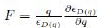 is the elasticity of the demand elasticity. These equations allows to understand the impact of the shape of the consumption tax on its incidence.

Proposition 3. In the case of a closed Cournot oligopoly, a change in the consumption tax such that the elasticity ∈_T increases but the consumer price stay unchanged leads to:

(a) a decrease of the producer price

(b) an increase of the ֝scal revenue

Proof. Comparing to equilibria with the same consumer price q, and therefore the same marginal cost of production and the same demand elasticity, equation 6 shows directly that the producer price is lower when the elasticity of the consumption tax is larger. Q.E.D.

What appens at equilibrium may be represented  by  figure  3  of  the  monopoly case. The difference is that the producer price curve is no more T^–1[D^–1(y)] but it is T^–1[D^–1 (Y₀ +γny_i)]. Furthermore, increasing the elasticity of the tax function but decreasing the value of the taxe in order to keep the same fiscal revenue results in a decrease of the consumer price and an increase of the output. The change is not Pareto improving because  of profit decrease,  but it surely  increase the social surplus.

3.2. Free entry

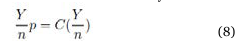
Seade (1980) introduced free entry in this kind of Cournot oligpoly. The equilibrium is characterized by the equation 6 of the maximization of profit and the equation 8 of zero profit because of the free entry.

In that case, an increase in the elasticity of the tax, even if it let the consumer price and the total output unchanged, modifies the number of firms and their individual production. However, the change in the producer price is notambiguous.

Proposition 4. In the case of a Cournot oligopoly  with  free  entry,  a  change  in  the consumption tax such that the elasticity ∈T increases but the consumer price stay unchanged leads to:

(a) a decrease of the producer price

(b) an increase of the ֝scal revenue

(c) a decrease of the number of ֝rms

(d) an increase of the output of each ֝rm

Proof.  Mixing  equations  6  and  8,  it  appears that equation 9 is verified at the equilibrium.

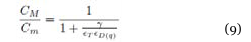
Where  C_m is the marginal cost of production and C_M the mean cost. As 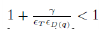 the mean cost is largerthan the marginal cost, which mean that the mean cost is decreasing with respect to output. With the assumption that the marginal cost does not decrease with respect to output, the ratio  decreases with respect to output.

Equation 9 shows that it also decreases with respect the tax elasticity ∈_T . Hence, the output per firm y increases with respect to the tax elasticity. As the consumer price and the total output are constant, the number of firms decreases. In addition, the free entry condition 8 establishes that the producer price p is equal to the mean cost of production. As the individual output increases and the mean cost decreases, the producer price decreases. Q.E.D.

The graphical representation of this equilibrium  is  presented  figure  4.  In  that  case, the entry occurs in the market whenever postive  profit  remains.  Hence,  Y₀  increases and the anticipated producer price curve T^–1[D^–1(Y₀(n)γny_i)]  is translated downard such as it becomes tangent to the mean cost curve. When the elasticity of the tax function increases, the slope of this producer price curve decreases, so the the point of tangency move along the mean cost curve to a lower mean cost, which leads to a lower producer 
price.

As in the short run, there exists a way of increasing the elasticity of the tax function which allows to simultaneously increase fiscal revenue and output and decrease consumer  price.  The  difference  is  that  profit stay at zero level. The upper elasticity equilibrium dominates the lower elasticity equilibrium because the gains in terms of fiscal revenue and consumer surplus (due to consumer price decrease and consumption increase)  are  obtained  not  by  profit  decrease but by production cost decrease (less firms and therefore less fixed costs).

4. Differentiated products

Previous results are univoque: increasing elasticity of the tax function is welfare improving. However, an important dimension has been forgotten: the quality of goods and their heterogeneity. Indeed, in the long run, an increase of the elasticity of the tax function leads to less firms, which means less variety. If consumers' utility increases with the variety of consumption, it may leads to welfare decline. The present section aims at considering this through models of heterogenous production. First, a very general framework is considered, first in the short run (4.1) then in the long run (4.2). A general equilibrium model of monopolistic competition is endly studied (?? to understand the inuence of the variations of the relative love for variety with respect to overall consumption.

4.1. Differentiated products in the short run

First a very general Bertrand competition model is first consider, based on those used by Anderson et al. (2001a,b).
In this model, n firms produce differentiated goods with the same marginal cost c and the same fixed cost K. Each producer i faces a demand D(q_i; q_–i) wich is symmetric and depend negatively on the consumer price q_i of the variety i and positively on the consumer 
price q_–i of other varieties. The profit of firm i is given by equation 10.

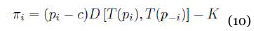
And the first order condition of the Bertrand-Nash equilibrium is given equation 11

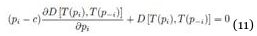
This problem is solved at the symetric equilibrium using the Chamberlain demand elasticities of curves dd and DD:

The elasticity of the slope of the dd  curve is . As in Anderson et al. (2001b), ∈DD > ∈dd and the stability condition is ∈dd + ∈DD – ∈m < 0.

Proposition  5. In the case of a Bertrand oligopoly in the short run, a change in the consumption tax such that the elasticity ∈T increases but the consumer price stay unchanged leads to:

(a) a decrease of the producer price

(b) an increase of the fiscal revenue

Proof.  The  first  order  condition  applied at the symetric equilibrium gives 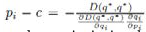. Consequently, the producer price is given by equation 12.

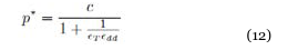
Hence, the producer price decreases with respect to the tax elasticity. Q.E.D.

4.2. Differentiated products in the long run

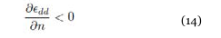
This general model of Bertrand oligopoly is more complex to solve in the long run. In particular, additional hypotheses sould be assumed, mainly regarding the way the demand evolve with respect to the number of varieties present on the market. The model is first modified by the addition of the variable n  of  the  number  of  firms  in  the  demand function for each firm: D (q_i; q_–i; n) with the hypothesis that the demand for each variety decreases with respect to the number of firms: An additional hypothesis sould be assumed, which is that competition lower prices: the consumer price q should decline with respect to the number of firm. Anderson et al. (2001b) demonstrate that this hypothese is equivalent to condition 13.

Where  is the elasticity of the dd curve slope with respect to n. Condition 13 may be expressed in terms of the variations with respect to the number of varities of the elasticity of the dd curve, as presented in condition 14.

Indeed, 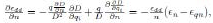 and therefore – as the elasticity of the dd curve is negative – this elasticity decreases with respect to the number of Érm if and only if  This result is very intuitive: when the number of varieties increases, the possibilities of substitutions are larger and the consumers are more elastic.

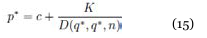
Two equations are needed to solve the equilibrium, the Érst order condition 12 and the zero proÉt condition 15.

However, the impact of ∈T on the producer price is less transparent in the present case. Previously, ∈dd (or ∈_q for the homogenous case) was invariant because the change of elasticity of the tax function was operated at constant consumer price q. Now, the demand – and consequently the demand elasticity – depends not only on the consumer price q but also on the number of varieties, which is not constant anymore. Therefore, the variation of the producer price depends on the derivative of the product ∈_T ∈_dd with 
respect to the change of the elasticity of the tax function.

The variation of the producer price occurs in the same way as those of this product (e.g.: equation 12). The variation of the demand fo a given Érm occurs in the opposite direction as those of the producer price (e.g.: equation 15), and therefore in the opposite direction as those of the product ∈_T ∈_dd. The variation of the number of Érms occurs in the opposite direction as those of the demand for a given Érm (because ∈n is negative), and therefore in the same way as those of the product ∈_T∈_dd. The derivative of this product with respect to the elasticity of the tax function (at constant consumer price q) may be expressed as in equation 16.

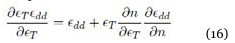
Hence, the product ∈_T∈_dd is decreasing with respect to ∈_T, which could be demonstrated by reductio ad absurdum. If were positive so would be  (following arguments of the previous paragraph). In addition, ∈_dd is negative and ∈_T is positive. Furthermore, condition 14 of the deationnist effect of competition states that is negative.

Consequently, both terms of the right hand side of equation 16 would be negative and so would be 

From these results may be derived the variations of the model' parameters when the elasticity of the tax function is increased in a such way that the consumer price keeps unchanged: the producer price diminishes and the number of varieties are reduced and the demand for each remaining Érms increases. As the total output Y is the product of the number  of  Érms  and  the  individual  demand  they face, this total output increases if ∈_n < –1 and decreases if ∈_n > –1. For the following, condition 17 is assumed.

The fact it is negative have been assumed earlier. The assumption of ∈_n being larger than –1 comes from the love for variety hypothesis. The inequality ∈_n < –1 would imply that the global demand for the whole varieties of a good increases when the number of varieties is reduced at constant consumer prices. In that case, consumer dislike variety.

Proposition  6.  In the case of a Bertrand oligopoly in the long run, if hypotheses 13 and 17 are veriɡed, a change in the consumption tax such that the elasticity ∈_T increases but the consumer price stay unchanged leads to:

(a) a decrease of the producer price, the number of ɡrms and the total output

(b) an increase of the demand per remaining ɡrm

(c) an increase then a decrease of the ɡscal revenue: there exists a positive and ɡnite elasticity of the tax function which maximizes the ɡscal revenue at constant consumer price.

Proofs The (a) and (b) results have been demonstrated previously. As a matter of the fiscal revenue FR, it is the product of the of the unitary tax t = q – p and the total output Y. Yet, Y = nD, so .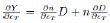

Due   to   the   definition   of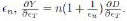  

Furthermore, condition 15 implies that 

It follows that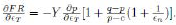 

Fiscal revenue increases if and only if the terme between brackets is positive.

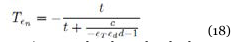
This defined a threshold T_∈n: when ∈_n is lower  than  this  threshold,  fiscal  revenue increases and it decreases when ∈_n > T_∈n. This threshold is given by equation 18.

Previous results show that both –∈_T∈_dd and the unitary tax t increases with respect to ∈_T at constant q. Therefore,there threshold decreases with respect ∈_T keeping between 0  and  1. When ∈T is low, the threshold is close to zero and greater than ∈_n (because of condition 17): the fiscal revenue increases with the increase of the elasticity of the tax function. However, with this increase, the threshold get closer to –1, eventually being lower than ∈n (also because of condition 17): the fiscal revenue decreases with the increase of the elasticity of the tax function. Q.E.D.

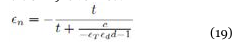
The optimal elasticity of the tax function (in  terms  of  fiscal  revenue  at  constant consumer price) is then obtained when condition 19 is verified.

This optimal elasticity of the tax function maximizes  the  scal  revenue  at  constant consumer price, but it does not maximizes the consumer surplus. Indeed, consumers purchase at the same price a quantity globally lower of less varieties of goods.

5. Conclusion and comments

This paper provides three kinds of contributions. From a methodological point of view it shows how to take the shape of the tax into account in order to derive the incidence of consumption taxes. The elasticity of the tax function which is the elasticity of the consumer price to the producer and depends only on the tax schedule. It enters in a tractable manner in inperfect competition models as the ratio of price elasticity of demand from the point of view of producers and consumers.

From a theoretical point of view, it generalizes existing results on the incidence of consumption taxes, up to now limited to ad valorem and per unit consumption taxes. In imperfect competition markets, the consumer share (producer share) of consumption taxes increases (decreases) with respect to the elasticity of the tax function. When it does not change the quality or diversity of output (e.g.: markets for homogenous goods or closed markets for heterogenous goods) the eciency of consumption tax is unambiguously increased by a larger elasticity of the consumption tax. However, the optimality of larger elasticity of the tax function is ambiguous when it changes the quality or diversity of output (e.g.: open markets for heterogenous goods). There exists a finite elasticity of the tax function maximizing the fiscal revenue at given consumer price (or minimizing consumer price at given fiscal revenue), but it is not optimal from the consumer point of view as it does not maximize the diversity of production.

Higher elasticities of the tax function are clearly welfare diminishing. Lower elasticities of the tax function (at fiscal revenue given) increase both consumer price and diversity of production, opening the question of arbitrage between price and diversity.

From an applied public economic point of view, this article shows how the regulator may put downwards prices on inperfect competition markets by increasing the elasticity of the consumption tax on a targeted window of producer prices. As shown by welfare ambiguity on competitive markets for heterogenous goods, this kind of policy should be limited to very uncompetitive markets. In the extreme case  of  infinite  elasticity  of  the  tax  function, the fiscality is equivalent to full price control. With finite but greater than one elasticities of the tax function, fiscal authority may perform partial price control through incentives. Keeping effective tax rates at realistic and non prohibitive levels forbids to increase the elasticity of the tax function for all possible prices: the large elasticities should target plausible prices inside producer price windows. The width of this large elasticity windows and the level of the elasticity are negatively linked.

The question of the arbitrage between prices and variety remains. In order to answer it, additional assumption should be made and the different models should be studied. First of all, it is of main concern, not only to catch the love for variety but also to model the way this love for variety evolves with respect to quantities consumed.

Those modeling already appeared in Dixit and Stiglitz (1977) when they relaxe the CES utility hypothesis. It is the objective of Kokovin et al. (2011) to provide a full model of monopolistic competition in general equilibrium without hypothesis on the variation of this love for variety. It should be relevant to study the arbitrage between price and diversity in their framework from a welfare point of view.

This would enlight this arbitrage from an individual perspective. It should also matter to understand this arbitrage in a distributive point of view. Actual consumers are heterogenous in matter of taste as much as in mater of wealth. Wealth differences should induces differences in the arbitrage between price and diversity of production. In that way, the choice of the elasticity of the tax function matters for the redistribution of welfare between households of different wealth. This should be studied through models with heterogeneity of consumer wealth. In addition, such studies should also point out the diversity in terms of quality of goods by the incidence of the elasticity of the tax function on the vertical diversity of goods. This should also raised some redistributive issues.